This article explains how to use the Compartments operation with imported Atlas objects to get segmentation results per atlas regions.
Background
Anatomical atlases are valuable tools in contextualizing segmentation results by allowing users to not only get object counts and morphologies, but also knowing how these change in various regions of an organism or organ. This article does not show how to import and register atlas objects to a sample dataset but only covers how to use pipelines that take imported atlas objects together with image segmentation to contextualise the information.
Analysis Pipeline
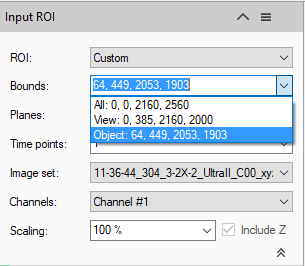
As always, the first step in the pipeline is the selection of the Input ROI. To speed up the pipeline it is generally advised to limit the analysis only to a specified region of interest. In this case this may involve restricting it only to the bounds of specific regions or the whole atlas. In our example, the atlas regions have already been imported as objects and so we can use the bounds of these objects in XY together with their extent in Z to set the input ROI. The bounds and plane range will depend on which objects are selected, whether just the one, a few, or all of them.
If any voxel operations are required to facilitate the segmentation these can be added to the pipeline prior to any segmentation step.
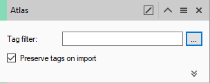
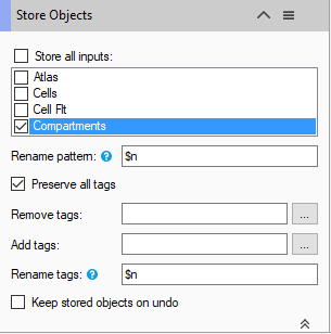
To use the atlas objects for compartmentalization they must be imported into the pipeline, Here we've used the Import Document Objects operation. Because there are no other objects in the dataset at present the Tag field can be left empty, otherwise, tags can be used to specify exactly which objects need to be used. We've also renamed the operation to "Atlas" so that all the objects get this tag to facilitate reading further pipeline operations.
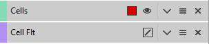
From there on we can segment and filter any of the objects that we want to compartmentalise. In our example we've used a blob finder segmentation and further filtered those objects to more specifically identify cells, but any segmentation tool can be used with whatever filter is required.
Having segmented all the objects to be compartmentalised, the final step is to group objects to their specific atlas regions. This is done using the Compartments operation.
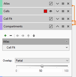
Object tags are added to the pipeline using the green "+" sign and arranged in order of hierarchy using the arrows. In the example above the objects with the tag "Cell Flt" have been configured to be children of Objects with the tag "Atlas". The threshold of inclusion has be set up so that if at least 50% of any object with the tag "Cell Flt" is within the boundary of an object with the tag "Atlas" it will become a child of that object.
Finally, as with any pipeline, we must save the objects.
Analysis Results
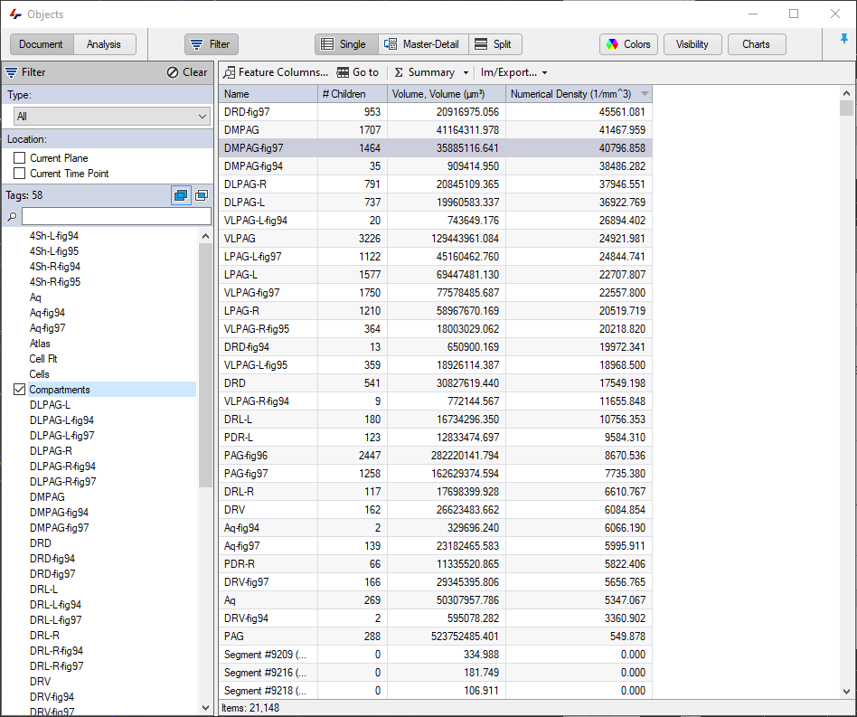
The results fo the pipeline are compartmentalised objects. There are several ways to review and interpret the data in the Objects table. Selecting the "Atlas" tag will display all the atlas objects and their features, which could include any morphological features of the objects (volume, surface area, sphericity, etc.), but can also include data concerning the children objects compartmentalized within them, such as the number of children, but also statistical values like numerical density which can be defined as a custom feature by dividing the number of children by the volume of the parent.
The objects table can also be arranged in the so called "Master-Detail" view where parents, track or groups appear in the top part of the table, and the children of these appear in the bottom. In such a layout it is then possible to view not just features of the groups, but also of the objects within them.
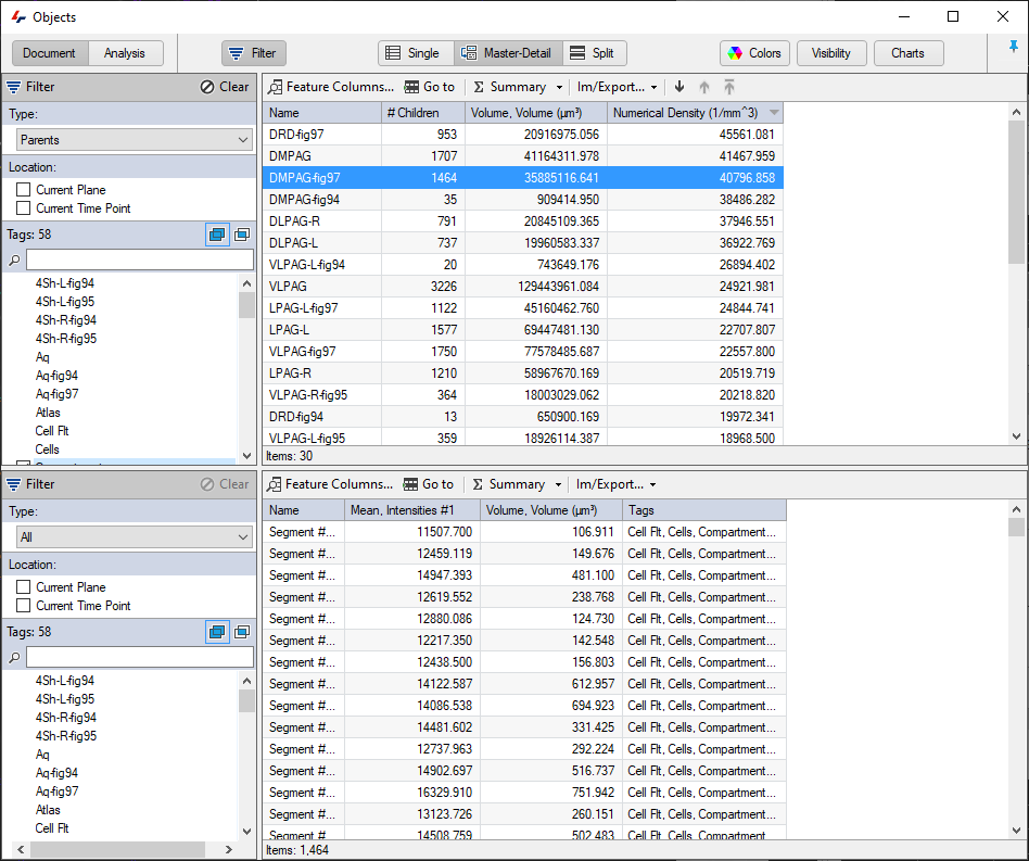
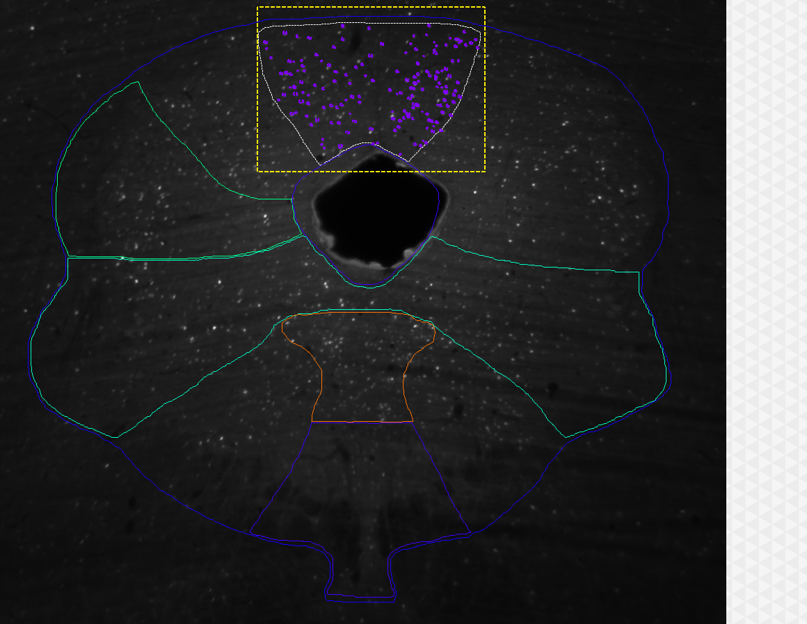
image courtesy: Kirsty Craigie, University of Edinburgh, UK.