Resolution is a term that is talked about a lot in imaging, but its meaning can vary depending on the context. This article seeks to clarify the meaning of resolution in the context of microscopy, specifically for image analysis.
Introduction
The Wiktionary lists 14 separate definitions for "resolution". In microscopy resolution is mostly related to the ability of the optical system to separate fine features clearly. In photography, resolution is used to measure the number of pixels in a camera sensor. In Imaging, resolution is something in between. It is formally defined as "the ability to separate the constituent parts of a whole".
In imaging, resolution is mostly defined by the following 4 factors:
- Optical resolution - how finely the optics separate points of light from their neighbors
- Sampling resolution - how finely the pixels on the camera sensor are separated
- Signal-to-noise ratio - how much light are we collecting compared to the noise generated by the system
- The bit depth of the imaging sensor - the degrees of separation between the minimum and maximum value recorded by the imaging device
The different types of resolution
Optical resolution
Whole books have been written on this topic by experts in optics, engineering, physics, and microscopy. We cannot do this topic justice in the context of this KB. Essentially, optical resolution is defined by the numerical aperture of the lens and the wavelength of light we are measuring. It is calculated slightly differently depending on whether we are working with transmitted light or fluorescent light, but in short, a higher NA for the objective lens generally means less blurring of the light and therefore better separation of the signal from the sample. Individual points of light projected through a lens are distorted into what is called an airy disc. The diameter of the airy disc limits the separation at which it becomes impossible to reliably tell 2 points of light apart.
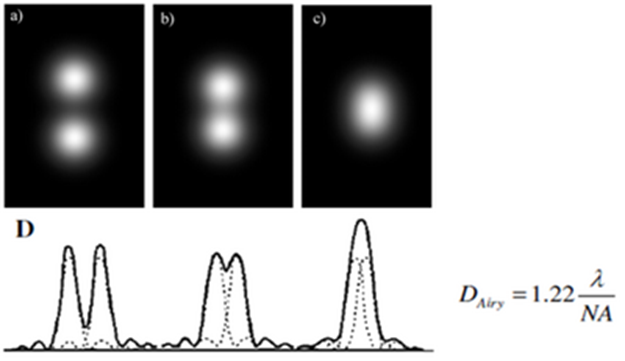
In fluorescence microscopy, the diameter of the airy disc is usually measured by the Rayleigh criterion. We can see from this formula that the shorter the wavelength of light or the higher the NA the smaller the diameter of the airy disc and the closer points of light can get to each other before we stop being able to tell them apart.
Sampling resolution
Imaging systems aren't made of just optical elements. To generate an image, we also need a sensor. In many optical systems, this sensor is a digital camera device, typically based on either CCD or CMOS technology, where the light is projected on a grid of individual light sensors we call pixels ("pixel" is a contraction of picture element). In laser scanning confocal we use a single light sensor and scan the sample using a laser then measure the light emission at regular intervals.
In either case, the light coming from the sample is not measured in a continuous fashion, but at specific intervals. The separation between those measurements is what we call the sampling resolution.
Because of this, the ability to resolve objects from an image isn't limited by the optics alone, it is also limited by the sampling frequency. If the inter-pixel separation is equivalent to 1um when we project light from the sample onto the sensor, the smallest gap we can measure will be larger than this since we need at least 1 pixel of separation to know a gap exists reliably. Likewise, if we are looking for fine features of 1um width in the sample, we really need a sampling frequency of at least half of that. In camera systems, the sampling frequency is the pixel separation on the silicon in the sensor / overall magnification of the optics. This number also serves as a calibration for the size of features in the image. A 10x lens paired to a camera with 5um pixel separation has a sampling resolution of 0.5um.
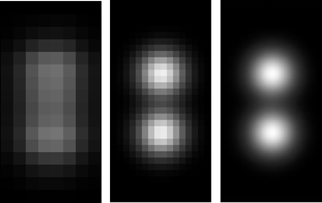
In this example above, the image on the left is under-sampled. It means that we cannot reliably say whether this is one continuous object, or two distinct objects that are in close proximity.
The image on the right is over-sampled. We can see the gap between the two objects, but the pixels are so fine that we have a lot more data to process, without getting any valuable information that might allow us to make significantly better measurements of the separation in the image.
The image in the middle is a good compromise between having the ability to still see the gap between the objects, with at least 2 pixels separating them, but without collecting so much information that we put an unnecessary burden on our computer to store and process the data.
Noise
While looking at resolution so far we have only considered ideal scenarios. In practice, images are never without noise. Noise can come from a variety of factors, including:
- Shot noise caused by the quantum nature of light
- Electronic noise from the imaging sensor we use to measure light, including read noise and dark current
- Out-of-focus light appearing at the plane we're imaging from points either further up or down the imaging axis
- Crosstalk or bleedthrough from different fluorophores from the on we are trying to measure
All of these, and their relative prominence relative to the signal we are trying to image, make up the signal-to-noise ratio. Let's look at how two of these work to better understand how they might affect our ability to separate objects.
When we measure the light coming from the sample, we usually have a system whereby a photon of light hits our sensor, and there is a given probability that this photon will excite an electron. Then, after a given period of time, we measure the voltage from the accumulated charge and we store this as a proxy for the intensity of the light emission intensity.
The probability that a photon will excite an electron is called the quantum efficiency. The excited electrons we measure are called photo-electrons. Shot noise comes from the fact that we may be measuring relatively few photons. If we have 10 photons of light hitting our sensor, with a quantum efficiency of 50%, it would not be uncommon to collect either 0 or 10 photo-electrons due to the probability that none of the photons manage to excite an electron or all the photons do. We could think of it as flipping a coin. From multiple series of 10 throws of the coin, we would expect the average to be 50/50 heads and tails, but it would not be that rare to end up with 10 heads in a row. However, if we take 1000 flips of the coin, the probability that none or all of them are heads diminishes towards 0. Likewise, as the number of photons we collect increases, the individual probability of error in the photo-electron count of individual pixels diminishes. Because of this, generally, the longer the exposure time, or the brighter the signal, the less noisy it will be.
At the same time, when we try to measure the accumulated charge from the excited photo-electrons, there is a certain degree of error in that measurement. We call this the read noise. When looking at specification sheets for cameras, the read noise is normally expressed as a number of electrons. If the read noise is 10 electrons, then we need to collect at least 10 more electrons in one pixel compared to its neighbor to reliably know that it collected more light. When we add the error in the measurement to the shot noise we get much closer to what you might actually expect from your imaging system.
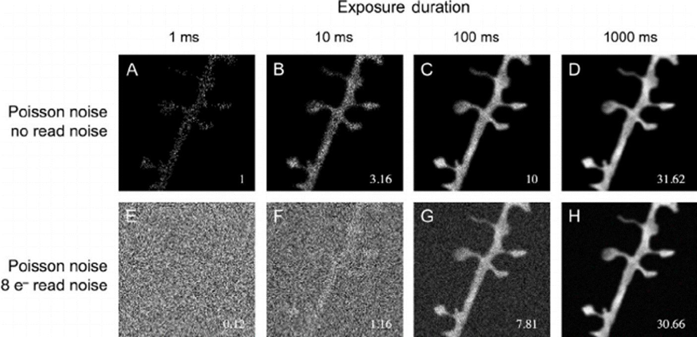
In the end, the main concern is whether the signal-to-noise ratio allows us to reliably see the connections or gaps between objects. In our example above, we can see the connection between the axon and the spines in the high-exposure image, but the noise in the 100ms image is too much to reliably know that they are connected. We could, with our knowledge of the sample and expected behavior tweak a segmentation pipeline to make it more likely to make that connection, but that would introduce a bias in our analysis that should be clearly stated when communicating these results.
Bit depth
Finally, we need to consider how computers store those intensity measurements.
Most will be familiar with the concept that computers store values as 1s and 0s. When storing image data, each pixel will represent a given number of bits that can be 1 or 0, the number of bits we use to store the value is called the bit depth.
An image with a bit depth of 1 will have 1 bit per pixel, so each pixel in the image will be either 0 or 1. If we had 2 bits, each pixel can be 00, 01, 10, or 11. Those binary numbers aren't very intuitive for humans, so we instead translate this as 0, 1, 2, and 3. As we increase the number of bits, we increase the range of values by 2 to the power of the bit depth. So, in a 4-bit image, we can have 2^4 = 16 degrees of variation, and if a pixel collected no light it would have a value of 0 and if it collected as much light as we're able to collect its value would be 15.
What does this mean for our digital camera images? As we saw, if we have a read noise of 10 electrons we need more than 10 electrons difference to know that a pixel is truly brighter. Our camera might have the capacity to store up to 10 000 electrons per pixel. We call this the full well capacity. If our camera's full well capacity is 10 000 electrons, and our read noise is 10 electrons, the degree of variation accuracy is 10 000 / 10 = 1000. So this camera could reliably measure 1000 levels of intensity, and we call this the dynamic range of the camera. 1000 isn't an exact power of 2, so instead we would most likely store the image in 10-bit, or 1024 greyscales, with the remaining 24 greyscales not making a significant difference to the overall accuracy of the measurement.
However, for a variety of reasons, computer data structures are easier to handle if they are made up of groups of 8 bits. So the most common image file formats usually store the intensity data as either 8 or 16-bit.
8-bit gives us 256 greyscales, for values going from 0 to 255. This is not a lot compared to the 1000 greyscale dynamic range of the sensor we just discussed above, but it is also roughly twice as good as the human eye can normally manage. In fact, because of this, most computer displays are limited to 8-bit display ranges, and conversely, higher bit depth images are displayed with this 8-bit display range.
With this in mind, we might ask what the utility is of storing the images in 16-bit, and this brings us back to what we mentioned earlier about measuring low levels of light.
A camera with a full well capacity of 10000 electrons and a read noise of 10 electrons might be OK for a brightfield system where we are collecting a lot of light, but a high-end fluorescence imaging sensor for low light imaging might more likely have a full well capacity of 80 000 electrons and a read noise of 2 electrons, which would give us an effective dynamic range of 40 000 greyscales. However, in low light imaging scenarios, the exposure time required for the highest intensity pixel to collect 80 000 photo-electrons might be measured in seconds. Exposing our sample for that length of time will probably be impractical for a range of reasons:
- our sample might be very dynamic and might move or change during that time
- such long exposure time might cause our excitation light to bleach the sample or kill it through photo-toxicity
- waiting several seconds to take a single snapshot would also make the acquisition of multiple Z planes less practically feasible
For all these reasons we might compromise and settle for a much shorter exposure time.
So, let's consider a case where we might have an ideal exposure time of 10s to collect 80 000 in at least 1 pixel. Instead, we might compromise and choose a 100ms exposure time and only collect 800 photo-electrons or 1/100th of the maximum intensity range. If we stored this image in 8-bit, we would only have 2, maybe 3, greyscales. If we stored these images in 16-bit instead, we would have 600 greyscales, and measurements of the difference between the brightest and darkest pixels in the image would be a lot more precise.
So, in the end, we store the images in 16-bit, not because we expect to accurately differentiate between 65 536 levels of intensity accurately, but because we might only collect a small fraction of the maximum intensity range and we still want to be able to work with that.
Conclusions
We discussed a lot of factors that affect what image analysts call resolution, but in the end, the consideration of what is useful resolution is fairly simple. We just need to ask ourselves the question:
When looking at the image at the pixel level, can I reliably identify the links connecting objects or the gaps separating them?
If we can answer that question in the positive then we can say that we have enough resolution in the image. If not, then considering the factors above should help in formulating a strategy to try and improve the resolution of our images. Of course, in the end, some compromises will most likely be required, but we should then be in a better position to judge the limitations of the analysis capabilities.