How does arivis handle large datasets

arivis solutions are known for their ability to handle large datasets. This article explains in a little more detail why and how this is done.

How do computers process image data?

Most people are familiar with the basic concept that computers deal with binary data, where every morsel of information that is stored and processed in a computer is reduced to a series of 1s and 0s. However, few truly understand how that affects many aspects of how computers store and process data. A complete explanation of the intricacies of computer data processing is much too large for the scope of this article, but some basic explanation may help clarify why arivis solutions do the things they do the way they are done.

The first thing to consider is how images are stored. Most will be familiar with the concept of Pixels. A pixel is very simply an intensity value for a specific point in a dataset. 

Looking at the example above, most human beings will, with little thought or effort, recognize a picture of an eye. But the data that is stored and displayed by the computer is a matrix of intensity values. What imaging software does is translate the numbers representing intensity values stored in the image file and display them as intensities on the screen for the purpose of visualization, or apply rules to individual pixels based on those intensity values to identify specific patterns like recognizing objects. To translate it into a more familiar concept, an image is essentially a spreadsheet of intensity values. 

Now, to come back to the idea of computers as binary machines that process 1s and 0s, these pixels values need to be stored in a way that makes sense to the computer. The smallest amount of information that a computer can process is called a bit. It is a value that can be either on or off, 1 or 0. Of course, when talking about intensity values, 1 or 0 is a very narrow range of possibilities. So, instead of using just one bit of data to store a pixel, we will use multiple bits. So, for a 2-bit image, each pixel would be represented by two bits. Therefore the completer range of possibilities would be 00, 01, 10, and 11. This gives us 4 degrees of variation. Each time we add a bit to our data structure we double the range of possible values. The more bits we use, the more degrees of separation we have between the minimum and maximum value.

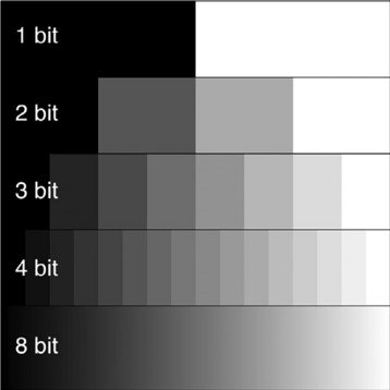But each bit also represents a certain amount of computing resource used to store and process the data contained therein. So, for example, an 8bit image gives us 2^8 degrees of intensity variation for intensities between 0 and 255,  and requires 8 bits or one byte per pixel in the image to store the file. In contrast, a 16-bit image gives us 2^16 degrees of variations (intensities between 0 and 65535), but also requires twice as much space on the disk and twice much processing resources as the 8-bit image since we are using twice as many bits to store and process the data. 

This is important because all the image processing will be done by the computer, which has limited resources, and the data that is being processed needs to be held in the system's memory (RAM) for it to be available to the CPU. Moreover, the memory not only needs to hold the data the CPU is processing, but also the result of those operations, meaning that the computer really needs at least twice as much RAM as the data we are trying to process. 

Typically in data processing, when an application opens a file, the entirety of that file's data is loaded into the system memory. Any processing on that image then outputs the results to the memory, and when the application closes only the necessary information is written back to the hard disk, either as a new file or modifications to the existing files. The problem with this approach comes when the files to be processed grow beyond the available memory. This is a very common problem in imaging as it is very easy when acquiring multidimensional datasets to generate files that are significantly larger than the available memory. Remember that each pixel usually represents 1 or 2 bytes of data. If we use a 1 million pixel imaging sensor, each image will represent 1/2 megabyte of data. If we acquire a Z-stack, we can multiply that by the number of planes in the stack. If we acquire multiple channels, as is common in fluorescence microscopy, we multiply the size of the dataset by the number of channels. If we want to measure changes over time we need to capture multiple time points. Each time we multiply the size of any of these dimensions we also multiply the size of the dataset by the same factor. It is relatively trivial in today's microscopy environment to generate datasets that represent several Terabytes of data. 

So what can we do to optimize the processing of such potentially large datasets?

Generally, in computing, there are a few specific bottlenecks that limit the ability to view and process data. These are:

• The number of display pixels - Most computer systems only have between 2 and 8 million pixels of screen real estate. A larger display with more pixels will also typically require more memory and a better GPU.
• Amount of memory available to the system - Most computers come with 8-16GB of memory as standard. High-end workstations can be configured with up to 2-4TB of memory, but these workstations will typically cost 10s of thousands of dollars, of which the memory could be as much as 2/3rds of the cost. 
• Central Processing Unit capabilities - Processing power is generally limited by several factors, from clock speed to core architecture. A common strategy to boost computing power is to use parallelization to split the processing across multiple cores. Not all tasks can be parallelized. 
• Graphics Processing Unit capabilities - GPUs are essentially small computing units inside your computer dedicated to the task of displaying information in 3D. They also have limitations with regards to the number and speed of the cores that can be built into a chip, and the amount of video memory available.
• Read/write speeds and storage capacity - As we'll see below, we can use temporary documents on the hard disk to work around memory limitations, but hard disks read/write speed can become important, especially when considering the cost/speed/capacity compromise for differing storage technologies. Also, many file formats don't readily allow a program to load only part of a file. 

First, in terms of pure visualization, as mentioned above most computer displays only have 2 to 8 million pixels of display real estate. When a TB image is loaded, it is almost impossible to physically display every pixel from the dataset on the screen at one time. Therefore, a system that spends minutes or hours loading the entire image in memory to only display a small fraction of these pixels at any one time is generally wasteful. Instead, arivis built a system that only loads the pixels that we need, at the resolution we need, as and when we need them.

Typically this is done by creating a so-called pyramidal file structure, where the image is stored with multiple levels of redundancy with regard to zoom levels, so that when you load the image at the lowest zoom level you only load the lowest resolution layer, and as the user zooms in we remove that from the memory and load the next layer with a higher resolution. This is generally very efficient with regards to memory use, but highly inefficient with regards to data storage as the pyramidal file can end up being 1.5x time larger than the raw data just to give this ability to load the resolution as needed. Instead, arivis uses a redundancy-free file structure where the resolution is calculated as needed, meaning that even without compression the converted SIS file will typically be as little as a few 100MB larger than the raw image data. On top of this, we can also apply lossless compression, of the same type as is used in standard compressed file formats like ZIP, to get between 20-80% compression ratios depending on the image data without any loss of information that is critical for scientific image analysis. 

When rendering a dataset in 3D, similar constraints exist with regards to the number of pixels that can be displayed on the screen, but also the rendering capabilities of the system are also going to be limited by the graphics capabilities of the GPU and the available video memory. So, likewise, when rendering in 3D arivis will first load in memory only as much of the image data as can be readily handled by the GPU to enable a smooth user experience. This leads to a small, but usually acceptable, loss in resolution for the purpose of interactive visualization and navigation. arivis Vision4D also gives the possibility to render at the highest level of resolution as and when needed and when user interactivity is no longer required.

When it comes to image processing, a simple workaround for memory availability is what is sometimes referred to as a divide-and-conquer approach or blocking. When using blocking, the software loads blocks of image data into the memory, then processes that block of data, and finally writes the results to a temporary document on the hard disk before loading the next block for processing. This very efficient method of processing does impose some constraints.

First, we need to have enough spare hard disk space to hold the processed images. However, since disk storage is generally significantly cheaper than RAM and there is usually a lot more of it available this is actually an asset of this approach. Our article outlining the system requirements for Vision4D has further details on this point. 

Second, a lot of image processing algorithms will be affected by the boundary pixels, meaning that we need to load a large enough margin on the side of the block we are interested in to allow for seamless stitching of the processed blocks.

Third, some image processing algorithms require the entire image to be held in memory. Therefore, as a result of our decision to make sure the software works with any images of any size on any computer we have specifically decided not to use these algorithms. 

And fourth, this approach requires a method of file access that permits the software to readily load arbitrary blocks of data from the file which not all files allow. To this end, arivis developed what we call arivis ImageCore. ImageCore is a combination of a file format that enables arbitrary access to any part of the file, and the libraries implemented in the software that allows us to make use of this feature. Because this is central to the way arivis solutions operate it also means that we do not *open* files such as TIFF, PNG, or any of the common microscopy imaging formats (CZI, LIF, OIF, ND2, etc), but instead we import the data contained in those files into a new file capable of storing all the information and make it accessible in a way that makes it readily accessible to our software.

The files that arivis creates use the ".SIS" extension. SIS files are multidimensional-redundancy free-pyramidal file structures with lossless compression support. This means that:

• We can load the resolution that we need to display the images as and when we need them without needing huge amounts of RAM
• We do so without adding a lot of redundant data to handle the different zoom levels, keeping the imported file size relatively small
• We can handle images of virtually infinite sizes in a range of dimensions. SIS files support virtually limitless numbers of channels, planes, time points, and tiles of any width and height. The only real limit is the size of the storage in your computer. SIS files are technically 7-dimensional, where each pixel can be anything from 8-bit to 32-bit floating-point, and each pixel belongs to a specific X, Y, and Z location in a specific channel, time point, and image set. 
• With lossless compression, we can further reduce the size of the imported file by 20-80% depending on the image data. 

So how does Vision4D work with my microscopy images?

Simply put, we don't. At least not directly. arivis Vision4D doesn't open any file in formats other than SIS. This means that to view and process your images we must first import them. To import a file into an SIS file we can simply drag and drop any supported file into an open viewer or our stand-alone SIS importer to start the import process. More details on the importing process can be found in the Getting Started user guide in the arivis Vision4D help menu. 

Once imported, the original file can be kept as backup storage for the raw data and the SIS file can be used as a working document for visualization and analysis. The importing process will, in most cases, automatically read and copy all the relevant image metadata (calibration, channel colours, time intervals etc). If some of the metadata is missing for any reason it can easily be updated and stored in the SIS file. SIS files support a range of storage features, including:

• Calibration information
• Time information
• Visualization parameters (colours, display range, LUTs)
• 3D Bookmarks (including opacity settings, clipping plane settings, 4D zoom and location...)
• Measurements (including lines, segments, tracks etc)
• Version history, allowing for undos even after closing and saving a file
• Original file metadata not normally used in image analysis (e.g. microscope parameters like laser power, lens characteristics, camera details etc)

Because the original file is left unchanged, users can work with SIS files in arivis Vision4D and VisionVR with full confidence that the original data is safe, that changes to the SIS file are reversible, and that the imported file can be opened and processed on virtually any computer that has enough storage space to hold the data.